
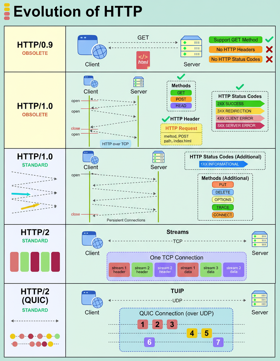
The Hypertext Transfer Protocol (HTTP) has undergone significant evolution to address the demands of contemporary applications, transitioning from basic text delivery to facilitating high-performance, real-time user experiences.
Its progression through various versions is outlined as follows:
An application programming interface (API) can experience slow performance. Determining the precise degree of slowness necessitates quantitative data—specific metrics that pinpoint malfunctions and guide rectification efforts.
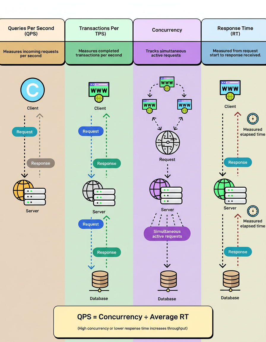
Key performance indicators that engineers should understand for comprehensive system performance analysis include:
Queries Per Second (QPS) represents the volume of incoming requests a system processes per second. For instance, a server receiving 1,000 requests in a single second demonstrates a QPS of 1,000. While seemingly simple, many systems struggle to maintain peak QPS levels over extended periods without encountering performance degradation or failures. This metric is crucial for understanding potential bottlenecks during high load events, such as those encountered during Black Friday Cyber Monday scale testing.
Transactions Per Second (TPS) measures the number of completed transactions a system processes within a second. A transaction encompasses the entire round trip, from an initial request, through database interaction, to the final response. TPS provides insight into the actual completed workload, distinguishing it from merely received requests, and is often a critical metric from a business perspective for tasks like Shopify BFCM readiness.
Concurrency indicates the number of simultaneous active requests a system is managing at any given instant. For example, if a system processes 100 requests per second, with each request requiring 5 seconds for completion, it effectively handles 500 concurrent requests. Elevated concurrency levels necessitate increased resource allocation, optimized connection pooling, and more sophisticated thread management strategies. This is especially relevant when considering capacity planning for large-scale applications.
Response Time (RT) defines the duration from the initiation of a request to the reception of its corresponding response. This metric is measurable at both the client and server levels. A fundamental relationship connects these metrics: QPS = Concurrency ÷ Average Response Time. Consequently, increased concurrency or reduced response time directly contributes to higher system throughput, a key consideration in effective capacity planning.
For two decades, Apache held a dominant position in the web server market. However, the introduction of Nginx brought significant advancements, leading to its adoption by some of the internet’s largest platforms, such as Netflix, Airbnb, Dropbox, and WordPress.com. Its widespread popularity stems not merely from its novelty or trendiness, but from its ability to efficiently address performance and scalability challenges that Apache struggled to manage.
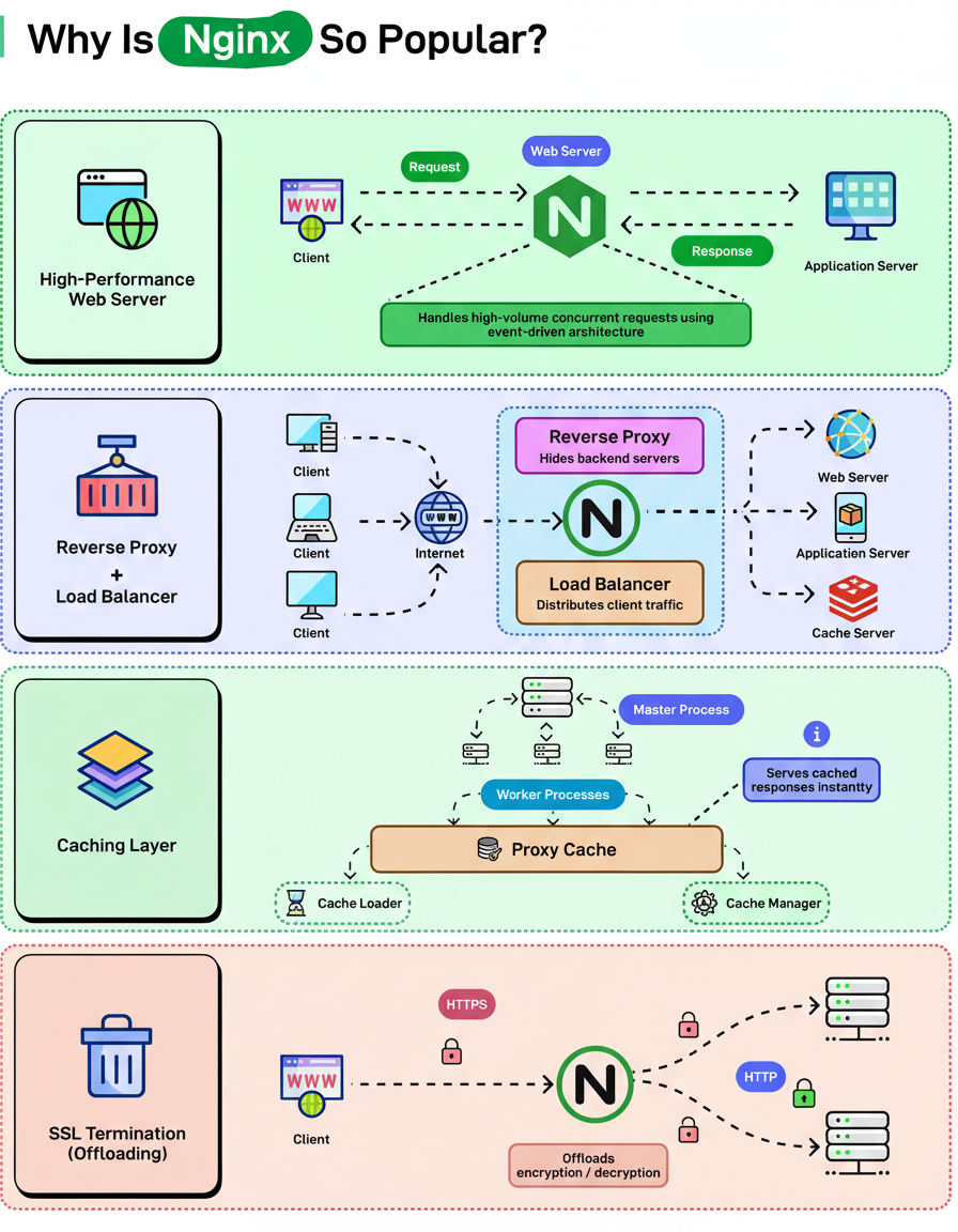
Several key attributes contribute to Nginx’s widespread acclaim:
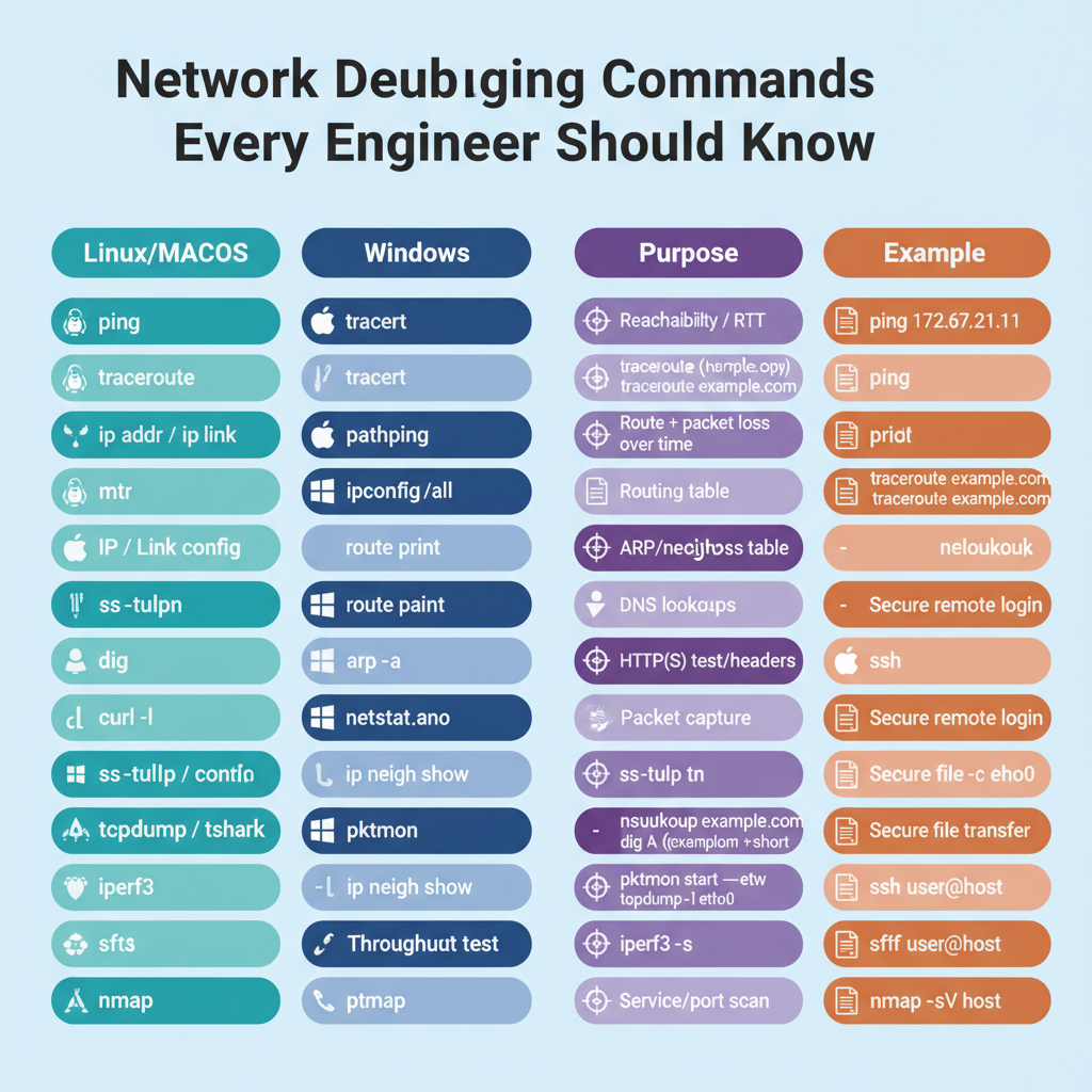
When confronted with a suspected network issue, specific diagnostic commands prove invaluable for rapid identification of the root cause.
Contemporary home and office networks universally depend on three fundamental devices: hubs, switches, and routers. Despite their ubiquitous presence, their distinct functions are frequently conflated.
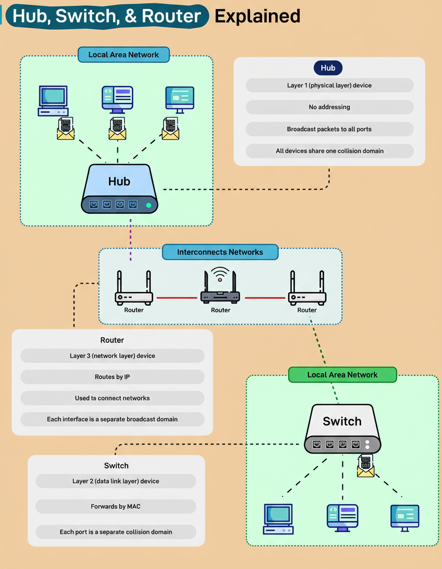
A hub functions at Layer 1 of the OSI model, the Physical Layer. Representing the simplest of these network devices, it lacks the ability to interpret addresses or data types. Upon receiving a packet, a hub merely broadcasts it to every connected device, thereby establishing a single, large collision domain. This operational characteristic implies that all connected devices contend for the same bandwidth, rendering hubs largely inefficient for contemporary network architectures.
Conversely, a switch operates at Layer 2, the Data Link Layer. It intelligently learns Media Access Control (MAC) addresses and selectively forwards data frames solely to their intended destination device. Each individual port on a switch constitutes its own collision domain, a design that significantly enhances efficiency and accelerates communication within a Local Area Network (LAN).
A router operates at Layer 3, the Network Layer. Its primary function involves routing data packets based on Internet Protocol (IP) addresses, effectively interconnecting disparate networks, such as a home network with the broader Internet. Each interface on a router establishes an independent broadcast domain, which serves to maintain isolation between local and external network traffic.
A comprehensive understanding of how these three networking layers collaboratively function forms the foundational knowledge essential for comprehending every modern network, ranging from residential Wi-Fi setups to the global Internet backbone.